Charting in Colaboratory
Contents
Charting in Colaboratory#
A common use for notebooks is data visualization using charts. Colaboratory makes this easy with several charting tools available as Python imports.
!pip install -q -r requirements.txt
Matplotlib#
Matplotlib is the most common charting package, see its documentation for details, and its examples for inspiration.
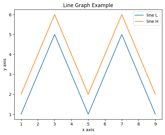
Line Plots#
import matplotlib.pyplot as plt

x  = [1, 2, 3, 4, 5, 6, 7, 8, 9]
y1 = [1, 3, 5, 3, 1, 3, 5, 3, 1]
y2 = [2, 4, 6, 4, 2, 4, 6, 4, 2]
plt.plot(x, y1, label="line L")
plt.plot(x, y2, label="line H")
plt.plot()

plt.xlabel("x axis")
plt.ylabel("y axis")
plt.title("Line Graph Example")
plt.legend()
plt.show()
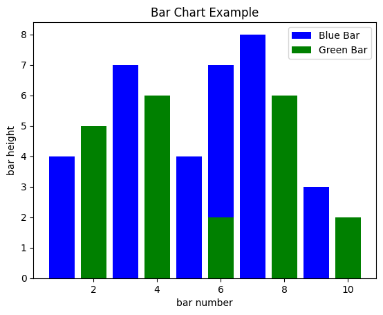
Bar Plots#
import matplotlib.pyplot as plt

# Look at index 4 and 6, which demonstrate overlapping cases.
x1 = [1, 3, 4, 5, 6, 7, 9]
y1 = [4, 7, 2, 4, 7, 8, 3]

x2 = [2, 4, 6, 8, 10]
y2 = [5, 6, 2, 6, 2]

# Colors: https://matplotlib.org/api/colors_api.html

plt.bar(x1, y1, label="Blue Bar", color='b')
plt.bar(x2, y2, label="Green Bar", color='g')
plt.plot()

plt.xlabel("bar number")
plt.ylabel("bar height")
plt.title("Bar Chart Example")
plt.legend()
plt.show()
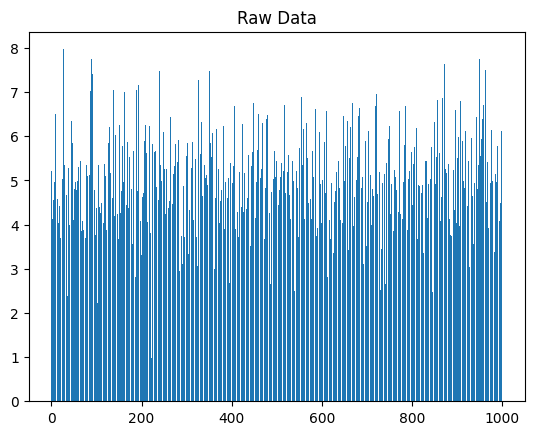
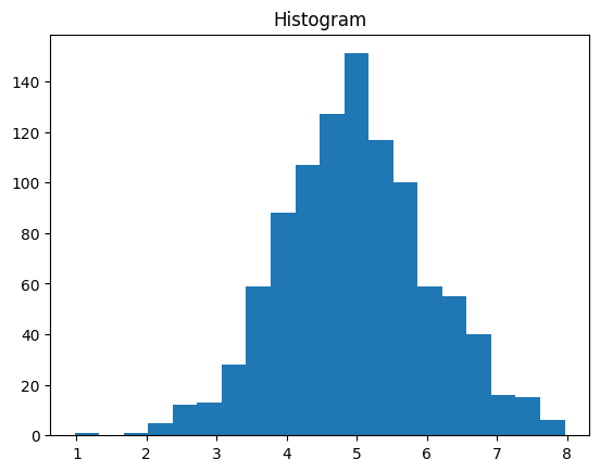
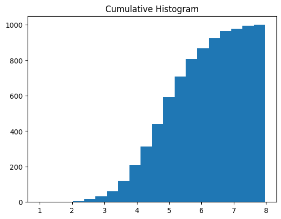
Histograms#
import matplotlib.pyplot as plt
import numpy as np

# Use numpy to generate a bunch of random data in a bell curve around 5.
n = 5 + np.random.randn(1000)

m = [m for m in range(len(n))]
plt.bar(m, n)
plt.title("Raw Data")
plt.show()

plt.hist(n, bins=20)
plt.title("Histogram")
plt.show()

plt.hist(n, cumulative=True, bins=20)
plt.title("Cumulative Histogram")
plt.show()
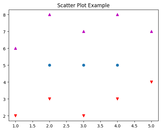
Scatter Plots#
import matplotlib.pyplot as plt

x1 = [2, 3, 4]
y1 = [5, 5, 5]

x2 = [1, 2, 3, 4, 5]
y2 = [2, 3, 2, 3, 4]
y3 = [6, 8, 7, 8, 7]

# Markers: https://matplotlib.org/api/markers_api.html

plt.scatter(x1, y1)
plt.scatter(x2, y2, marker='v', color='r')
plt.scatter(x2, y3, marker='^', color='m')
plt.title('Scatter Plot Example')
plt.show()
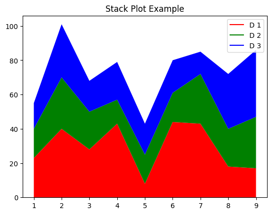
Stack Plots#
import matplotlib.pyplot as plt

idxes = [ 1,  2,  3,  4,  5,  6,  7,  8,  9]
arr1  = [23, 40, 28, 43,  8, 44, 43, 18, 17]
arr2  = [17, 30, 22, 14, 17, 17, 29, 22, 30]
arr3  = [15, 31, 18, 22, 18, 19, 13, 32, 39]

# Adding legend for stack plots is tricky.
plt.plot([], [], color='r', label = 'D 1')
plt.plot([], [], color='g', label = 'D 2')
plt.plot([], [], color='b', label = 'D 3')

plt.stackplot(idxes, arr1, arr2, arr3, colors= ['r', 'g', 'b'])
plt.title('Stack Plot Example')
plt.legend()
plt.show()
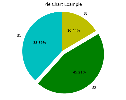
Pie Charts#
import matplotlib.pyplot as plt

labels = 'S1', 'S2', 'S3'
sections = [56, 66, 24]
colors = ['c', 'g', 'y']

plt.pie(sections, labels=labels, colors=colors,
        startangle=90,
        explode = (0, 0.1, 0),
        autopct = '%1.2f%%')

plt.axis('equal') # Try commenting this out.
plt.title('Pie Chart Example')
plt.show()
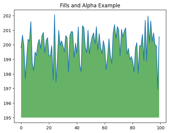
fill_between and alpha#
import matplotlib.pyplot as plt
import numpy as np

ys = 200 + np.random.randn(100)
x = [x for x in range(len(ys))]

plt.plot(x, ys, '-')
plt.fill_between(x, ys, 195, where=(ys > 195), facecolor='g', alpha=0.6)

plt.title("Fills and Alpha Example")
plt.show()
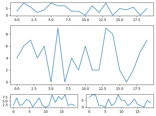
Subplotting using Subplot2grid#
import matplotlib.pyplot as plt
import numpy as np

def random_plots():
  xs = []
  ys = []

  for i in range(20):
    x = i
    y = np.random.randint(10)

    xs.append(x)
    ys.append(y)

  return xs, ys

fig = plt.figure()
ax1 = plt.subplot2grid((5, 2), (0, 0), rowspan=1, colspan=2)
ax2 = plt.subplot2grid((5, 2), (1, 0), rowspan=3, colspan=2)
ax3 = plt.subplot2grid((5, 2), (4, 0), rowspan=1, colspan=1)
ax4 = plt.subplot2grid((5, 2), (4, 1), rowspan=1, colspan=1)

x, y = random_plots()
ax1.plot(x, y)

x, y = random_plots()
ax2.plot(x, y)

x, y = random_plots()
ax3.plot(x, y)

x, y = random_plots()
ax4.plot(x, y)

plt.tight_layout()
plt.show()
Plot styles#
Colaboratory charts use Seaborn’s custom styling by default. To customize styling further please see the matplotlib docs.
3D Graphs#
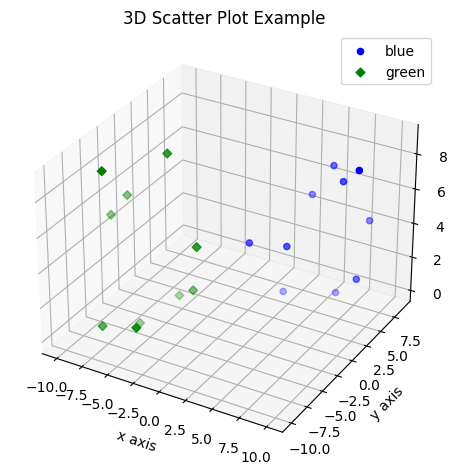
3D Scatter Plots#
import matplotlib.pyplot as plt
import numpy as np
from mpl_toolkits.mplot3d import axes3d

fig = plt.figure()
ax = fig.add_subplot(111, projection = '3d')

x1 = [1, 2, 3, 4, 5, 6, 7, 8, 9, 10]
y1 = np.random.randint(10, size=10)
z1 = np.random.randint(10, size=10)

x2 = [-1, -2, -3, -4, -5, -6, -7, -8, -9, -10]
y2 = np.random.randint(-10, 0, size=10)
z2 = np.random.randint(10, size=10)

ax.scatter(x1, y1, z1, c='b', marker='o', label='blue')
ax.scatter(x2, y2, z2, c='g', marker='D', label='green')

ax.set_xlabel('x axis')
ax.set_ylabel('y axis')
ax.set_zlabel('z axis')
plt.title("3D Scatter Plot Example")
plt.legend()
plt.tight_layout()
plt.show()
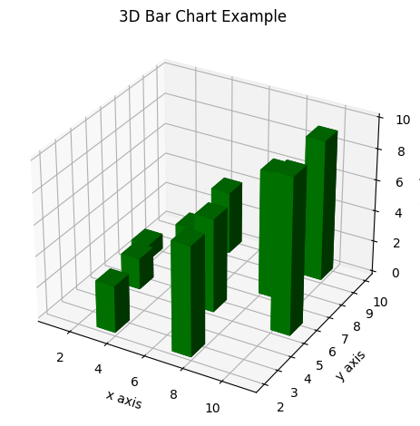
3D Bar Plots#
import matplotlib.pyplot as plt
import numpy as np

fig = plt.figure()
ax = fig.add_subplot(111, projection = '3d')

x = [1, 2, 3, 4, 5, 6, 7, 8, 9, 10]
y = np.random.randint(10, size=10)
z = np.zeros(10)

dx = np.ones(10)
dy = np.ones(10)
dz = [1, 2, 3, 4, 5, 6, 7, 8, 9, 10]

ax.bar3d(x, y, z, dx, dy, dz, color='g')

ax.set_xlabel('x axis')
ax.set_ylabel('y axis')
ax.set_zlabel('z axis')
plt.title("3D Bar Chart Example")
plt.tight_layout()
plt.show()
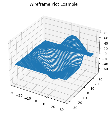
Wireframe Plots#
import matplotlib.pyplot as plt

fig = plt.figure()
ax = fig.add_subplot(111, projection = '3d')

x, y, z = axes3d.get_test_data()

ax.plot_wireframe(x, y, z, rstride = 2, cstride = 2)

plt.title("Wireframe Plot Example")
plt.tight_layout()
plt.show()
Seaborn#
There are several libraries layered on top of Matplotlib that you can use in Colab. One that is worth highlighting is Seaborn:
import matplotlib.pyplot as plt
import numpy as np
import seaborn as sns

# Generate some random data
num_points = 20
# x will be 5, 6, 7... but also twiddled randomly
x = 5 + np.arange(num_points) + np.random.randn(num_points)
# y will be 10, 11, 12... but twiddled even more randomly
y = 10 + np.arange(num_points) + 5 * np.random.randn(num_points)
sns.regplot(x, y)
plt.show()
C:\Users\schatzm\Anaconda3\envs\ju-book\Lib\site-packages\seaborn\_decorators.py:36: FutureWarning: Pass the following variables as keyword args: x, y. From version 0.12, the only valid positional argument will be `data`, and passing other arguments without an explicit keyword will result in an error or misinterpretation.
  warnings.warn(
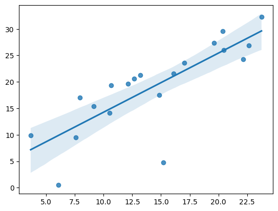
That’s a simple scatterplot with a nice regression line fit to it, all with just one call to Seaborn’s regplot.
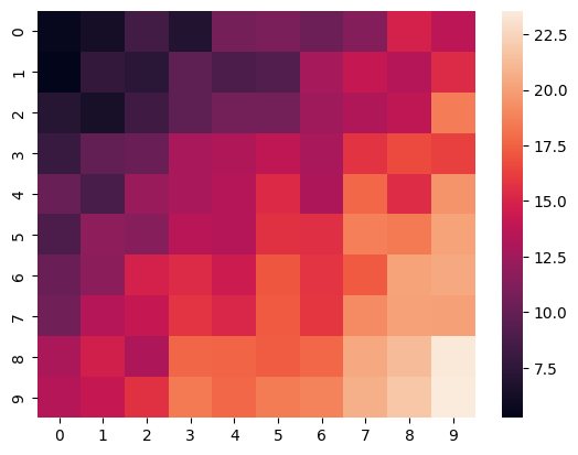
Here’s a Seaborn heatmap:
import matplotlib.pyplot as plt
import numpy as np

# Make a 10 x 10 heatmap of some random data
side_length = 10
# Start with a 10 x 10 matrix with values randomized around 5
data = 5 + np.random.randn(side_length, side_length)
# The next two lines make the values larger as we get closer to (9, 9)
data += np.arange(side_length)
data += np.reshape(np.arange(side_length), (side_length, 1))
# Generate the heatmap
sns.heatmap(data)
plt.show()
Altair#
Altair is a declarative visualization library for creating interactive visualizations in Python, and is installed and enabled in Colab by default.
For example, here is an interactive scatter plot:
import altair as alt
from vega_datasets import data
cars = data.cars()

alt.Chart(cars).mark_point().encode(
    x='Horsepower',
    y='Miles_per_Gallon',
    color='Origin',
).interactive()
C:\Users\schatzm\Anaconda3\envs\ju-book\Lib\site-packages\altair\utils\core.py:317: FutureWarning: iteritems is deprecated and will be removed in a future version. Use .items instead.
  for col_name, dtype in df.dtypes.iteritems():
For more examples of Altair plots, see the Altair snippets notebook or the external Altair Example Gallery.
Plotly#
Sample#
from plotly.offline import iplot
import plotly.graph_objs as go

data = [
    go.Contour(
        z=[[10, 10.625, 12.5, 15.625, 20],
           [5.625, 6.25, 8.125, 11.25, 15.625],
           [2.5, 3.125, 5., 8.125, 12.5],
           [0.625, 1.25, 3.125, 6.25, 10.625],
           [0, 0.625, 2.5, 5.625, 10]]
    )
]
iplot(data)
Bokeh#
Sample#
import numpy as np
from bokeh.plotting import figure, show
from bokeh.io import output_notebook

# Call once to configure Bokeh to display plots inline in the notebook.
output_notebook()
N = 4000
x = np.random.random(size=N) * 100
y = np.random.random(size=N) * 100
radii = np.random.random(size=N) * 1.5
colors = ["#%02x%02x%02x" % (r, g, 150) for r, g in zip(np.floor(50+2*x).astype(int), np.floor(30+2*y).astype(int))]

p = figure()
p.circle(x, y, radius=radii, fill_color=colors, fill_alpha=0.6, line_color=None)
show(p)
from watermark import watermark
watermark(iversions=True, globals_=globals())
print(watermark())
Last updated: 2023-01-05T14:38:25.736730+01:00

Python implementation: CPython
Python version       : 3.11.0
IPython version      : 8.8.0

Compiler    : MSC v.1929 64 bit (AMD64)
OS          : Windows
Release     : 10
Machine     : AMD64
Processor   : Intel64 Family 6 Model 85 Stepping 7, GenuineIntel
CPU cores   : 40
Architecture: 64bit
print(watermark(packages="watermark,numpy,pandas,matplotlib,bokeh,altair,plotly"))
watermark : 2.3.1
numpy     : 1.24.1
pandas    : 1.5.2
matplotlib: 3.6.2
bokeh     : 3.0.3
altair    : 4.2.0
plotly    : 5.11.0