Introduction to Pandas
Contents
Introduction to Pandas#
Copyright 2017 Google LLC.#
# Licensed under the Apache License, Version 2.0 (the "License");
# you may not use this file except in compliance with the License.
# You may obtain a copy of the License at
#
# https://www.apache.org/licenses/LICENSE-2.0
#
# Unless required by applicable law or agreed to in writing, software
# distributed under the License is distributed on an "AS IS" BASIS,
# WITHOUT WARRANTIES OR CONDITIONS OF ANY KIND, either express or implied.
# See the License for the specific language governing permissions and
# limitations under the License.
Intro to pandas#
Learning Objectives:
Gain an introduction to the
DataFrameandSeriesdata structures of the pandas libraryAccess and manipulate data within a
DataFrameandSeriesImport CSV data into a pandas
DataFrameReindex a
DataFrameto shuffle data
pandas is a column-oriented data analysis API. It’s a great tool for handling and analyzing input data, and many ML frameworks support pandas data structures as inputs. Although a comprehensive introduction to the pandas API would span many pages, the core concepts are fairly straightforward, and we’ll present them below. For a more complete reference, the pandas docs site contains extensive documentation and many tutorials.
Basic Concepts#
The following line imports the pandas API and prints the API version:
!pip install -q -r requirements.txt
from __future__ import print_function

import pandas as pd
pd.__version__
'1.5.2'
The primary data structures in pandas are implemented as two classes:
DataFrame, which you can imagine as a relational data table, with rows and named columns.Series, which is a single column. ADataFramecontains one or moreSeriesand a name for eachSeries.
The data frame is a commonly used abstraction for data manipulation. Similar implementations exist in Spark and R.
One way to create a Series is to construct a Series object. For example:
pd.Series(['San Francisco', 'San Jose', 'Sacramento'])
0    San Francisco
1         San Jose
2       Sacramento
dtype: object
DataFrame objects can be created by passing a dict mapping string column names to their respective Series. If the Series don’t match in length, missing values are filled with special NA/NaN values. Example:
city_names = pd.Series(['San Francisco', 'San Jose', 'Sacramento'])
population = pd.Series([852469, 1015785, 485199])

pd.DataFrame({ 'City name': city_names, 'Population': population })
| City name | Population | |
|---|---|---|
| 0 | San Francisco | 852469 |
| 1 | San Jose | 1015785 |
| 2 | Sacramento | 485199 |
But most of the time, you load an entire file into a DataFrame. The following example loads a file with California housing data. Run the following cell to load the data and create feature definitions:
california_housing_dataframe = pd.read_csv("https://download.mlcc.google.com/mledu-datasets/california_housing_train.csv", sep=",")
california_housing_dataframe.describe()
| longitude | latitude | housing_median_age | total_rooms | total_bedrooms | population | households | median_income | median_house_value | |
|---|---|---|---|---|---|---|---|---|---|
| count | 17000.000000 | 17000.000000 | 17000.000000 | 17000.000000 | 17000.000000 | 17000.000000 | 17000.000000 | 17000.000000 | 17000.000000 |
| mean | -119.562108 | 35.625225 | 28.589353 | 2643.664412 | 539.410824 | 1429.573941 | 501.221941 | 3.883578 | 207300.912353 |
| std | 2.005166 | 2.137340 | 12.586937 | 2179.947071 | 421.499452 | 1147.852959 | 384.520841 | 1.908157 | 115983.764387 |
| min | -124.350000 | 32.540000 | 1.000000 | 2.000000 | 1.000000 | 3.000000 | 1.000000 | 0.499900 | 14999.000000 |
| 25% | -121.790000 | 33.930000 | 18.000000 | 1462.000000 | 297.000000 | 790.000000 | 282.000000 | 2.566375 | 119400.000000 |
| 50% | -118.490000 | 34.250000 | 29.000000 | 2127.000000 | 434.000000 | 1167.000000 | 409.000000 | 3.544600 | 180400.000000 |
| 75% | -118.000000 | 37.720000 | 37.000000 | 3151.250000 | 648.250000 | 1721.000000 | 605.250000 | 4.767000 | 265000.000000 |
| max | -114.310000 | 41.950000 | 52.000000 | 37937.000000 | 6445.000000 | 35682.000000 | 6082.000000 | 15.000100 | 500001.000000 |
The example above used DataFrame.describe to show interesting statistics about a DataFrame. Another useful function is DataFrame.head, which displays the first few records of a DataFrame:
california_housing_dataframe.head()
| longitude | latitude | housing_median_age | total_rooms | total_bedrooms | population | households | median_income | median_house_value | |
|---|---|---|---|---|---|---|---|---|---|
| 0 | -114.31 | 34.19 | 15.0 | 5612.0 | 1283.0 | 1015.0 | 472.0 | 1.4936 | 66900.0 |
| 1 | -114.47 | 34.40 | 19.0 | 7650.0 | 1901.0 | 1129.0 | 463.0 | 1.8200 | 80100.0 |
| 2 | -114.56 | 33.69 | 17.0 | 720.0 | 174.0 | 333.0 | 117.0 | 1.6509 | 85700.0 |
| 3 | -114.57 | 33.64 | 14.0 | 1501.0 | 337.0 | 515.0 | 226.0 | 3.1917 | 73400.0 |
| 4 | -114.57 | 33.57 | 20.0 | 1454.0 | 326.0 | 624.0 | 262.0 | 1.9250 | 65500.0 |
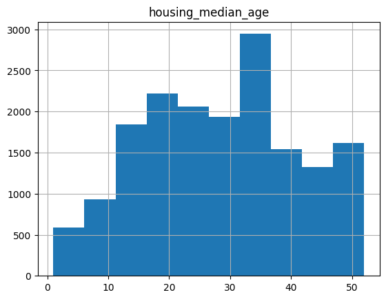
Another powerful feature of pandas is graphing. For example, DataFrame.hist lets you quickly study the distribution of values in a column:
california_housing_dataframe.hist('housing_median_age')
array([[<AxesSubplot: title={'center': 'housing_median_age'}>]],
      dtype=object)
Accessing Data#
You can access DataFrame data using familiar Python dict/list operations:
cities = pd.DataFrame({ 'City name': city_names, 'Population': population })
print(type(cities['City name']))
cities['City name']
<class 'pandas.core.series.Series'>
0    San Francisco
1         San Jose
2       Sacramento
Name: City name, dtype: object
print(type(cities['City name'][1]))
cities['City name'][1]
<class 'str'>
'San Jose'
print(type(cities[0:2]))
cities[0:2]
<class 'pandas.core.frame.DataFrame'>
| City name | Population | |
|---|---|---|
| 0 | San Francisco | 852469 |
| 1 | San Jose | 1015785 |
In addition, pandas provides an extremely rich API for advanced indexing and selection that is too extensive to be covered here.
Manipulating Data#
You may apply Python’s basic arithmetic operations to Series. For example:
population / 1000.
0     852.469
1    1015.785
2     485.199
dtype: float64
NumPy is a popular toolkit for scientific computing. pandas Series can be used as arguments to most NumPy functions:
import numpy as np

np.log(population)
0    13.655892
1    13.831172
2    13.092314
dtype: float64
For more complex single-column transformations, you can use Series.apply. Like the Python map function,
Series.apply accepts as an argument a lambda function, which is applied to each value.
The example below creates a new Series that indicates whether population is over one million:
population.apply(lambda val: val > 1000000)
0    False
1     True
2    False
dtype: bool
Modifying DataFrames is also straightforward. For example, the following code adds two Series to an existing DataFrame:
cities['Area square miles'] = pd.Series([46.87, 176.53, 97.92])
cities['Population density'] = cities['Population'] / cities['Area square miles']
cities
| City name | Population | Area square miles | Population density | |
|---|---|---|---|---|
| 0 | San Francisco | 852469 | 46.87 | 18187.945381 |
| 1 | San Jose | 1015785 | 176.53 | 5754.177760 |
| 2 | Sacramento | 485199 | 97.92 | 4955.055147 |
Exercise #1#
Modify the cities table by adding a new boolean column that is True if and only if both of the following are True:
The city is named after a saint.
The city has an area greater than 50 square miles.
Note: Boolean Series are combined using the bitwise, rather than the traditional boolean, operators. For example, when performing logical and, use & instead of and.
Hint: “San” in Spanish means “saint.”
# Your code here
Solution#
Click below for a solution.
cities['Is wide and has saint name'] = (cities['Area square miles'] > 50) & cities['City name'].apply(lambda name: name.startswith('San'))
cities
| City name | Population | Area square miles | Population density | Is wide and has saint name | |
|---|---|---|---|---|---|
| 0 | San Francisco | 852469 | 46.87 | 18187.945381 | False |
| 1 | San Jose | 1015785 | 176.53 | 5754.177760 | True |
| 2 | Sacramento | 485199 | 97.92 | 4955.055147 | False |
Indexes#
Both Series and DataFrame objects also define an index property that assigns an identifier value to each Series item or DataFrame row.
By default, at construction, pandas assigns index values that reflect the ordering of the source data. Once created, the index values are stable; that is, they do not change when data is reordered.
city_names.index
RangeIndex(start=0, stop=3, step=1)
cities.index
RangeIndex(start=0, stop=3, step=1)
Call DataFrame.reindex to manually reorder the rows. For example, the following has the same effect as sorting by city name:
cities.reindex([2, 0, 1])
| City name | Population | Area square miles | Population density | Is wide and has saint name | |
|---|---|---|---|---|---|
| 2 | Sacramento | 485199 | 97.92 | 4955.055147 | False |
| 0 | San Francisco | 852469 | 46.87 | 18187.945381 | False |
| 1 | San Jose | 1015785 | 176.53 | 5754.177760 | True |
Reindexing is a great way to shuffle (randomize) a DataFrame. In the example below, we take the index, which is array-like, and pass it to NumPy’s random.permutation function, which shuffles its values in place. Calling reindex with this shuffled array causes the DataFrame rows to be shuffled in the same way.
Try running the following cell multiple times!
cities.reindex(np.random.permutation(cities.index))
| City name | Population | Area square miles | Population density | Is wide and has saint name | |
|---|---|---|---|---|---|
| 0 | San Francisco | 852469 | 46.87 | 18187.945381 | False |
| 2 | Sacramento | 485199 | 97.92 | 4955.055147 | False |
| 1 | San Jose | 1015785 | 176.53 | 5754.177760 | True |
For more information, see the Index documentation.
Exercise #2#
The reindex method allows index values that are not in the original DataFrame’s index values. Try it and see what happens if you use such values! Why do you think this is allowed?
# Your code here
Solution#
Click below for the solution.
If your reindex input array includes values not in the original DataFrame index values, reindex will add new rows for these “missing” indices and populate all corresponding columns with NaN values:
cities.reindex([0, 4, 5, 2])
| City name | Population | Area square miles | Population density | Is wide and has saint name | |
|---|---|---|---|---|---|
| 0 | San Francisco | 852469.0 | 46.87 | 18187.945381 | False |
| 4 | NaN | NaN | NaN | NaN | NaN |
| 5 | NaN | NaN | NaN | NaN | NaN |
| 2 | Sacramento | 485199.0 | 97.92 | 4955.055147 | False |
This behavior is desirable because indexes are often strings pulled from the actual data (see the pandas reindex documentation for an example in which the index values are browser names).
In this case, allowing “missing” indices makes it easy to reindex using an external list, as you don’t have to worry about sanitizing the input.
Creating subsets#
d1Area = california_housing_dataframe[['population','households','median_income']]
d2Area=d1Area;
Filtering#
d1Area.dropna(how='all')
| population | households | median_income | |
|---|---|---|---|
| 0 | 1015.0 | 472.0 | 1.4936 |
| 1 | 1129.0 | 463.0 | 1.8200 |
| 2 | 333.0 | 117.0 | 1.6509 |
| 3 | 515.0 | 226.0 | 3.1917 |
| 4 | 624.0 | 262.0 | 1.9250 |
| ... | ... | ... | ... |
| 16995 | 907.0 | 369.0 | 2.3571 |
| 16996 | 1194.0 | 465.0 | 2.5179 |
| 16997 | 1244.0 | 456.0 | 3.0313 |
| 16998 | 1298.0 | 478.0 | 1.9797 |
| 16999 | 806.0 | 270.0 | 3.0147 |
17000 rows × 3 columns
Concat#
data1=d1Area.sample(n=500, random_state=1)
data1['Label']='Data1'

data2=d2Area.sample(n=500, random_state=1)
data2['Label']='Data2'

resultOut = pd.concat([data1, data2])
Reorder columns
data1=data1[['Label','population','households','median_income']]
data1.head()
| Label | population | households | median_income | |
|---|---|---|---|---|
| 4752 | Data1 | 2621.0 | 661.0 | 6.2427 |
| 13348 | Data1 | 1043.0 | 351.0 | 6.2048 |
| 13459 | Data1 | 619.0 | 231.0 | 4.6304 |
| 6691 | Data1 | 634.0 | 261.0 | 1.6406 |
| 12750 | Data1 | 3060.0 | 1060.0 | 5.3064 |
data2=data2[['Label','population','households','median_income']]
data2.head()
| Label | population | households | median_income | |
|---|---|---|---|---|
| 4752 | Data2 | 2621.0 | 661.0 | 6.2427 |
| 13348 | Data2 | 1043.0 | 351.0 | 6.2048 |
| 13459 | Data2 | 619.0 | 231.0 | 4.6304 |
| 6691 | Data2 | 634.0 | 261.0 | 1.6406 |
| 12750 | Data2 | 3060.0 | 1060.0 | 5.3064 |
Reading in data#
Let’s first look at the doc string of pd.read_csv().
pd.read_csv?
Saving data#
compression_opts = dict(method='zip',
                        archive_name='ResultArea_out500.csv')
resultOut.to_csv('resultOut.zip', index=False,
          compression=compression_opts)